Note
Go to the end to download the full example code.
Retrieving wind drift factor from trajectory
import trajan as _
from datetime import datetime, timedelta
import pandas as pd
import numpy as np
import matplotlib.pyplot as plt
import cmocean
from opendrift import test_data_folder as tdf
from opendrift.models.oceandrift import OceanDrift
from opendrift.models.physics_methods import wind_drift_factor_from_trajectory
A very simple drift model is: current + wind_drift_factor*wind where wind_drift_factor for surface drift is typically 0.033 if Stokes drift included, and 0.02 in addition to Stokes drift. This example illustrates how a best-fit wind_drift_factor can be calculated from an observed trajectory, using two different methods.
First we simulate a synthetic drifter trajectory
ot = OceanDrift(loglevel=50)
ot.add_readers_from_list([tdf +
    '16Nov2015_NorKyst_z_surface/norkyst800_subset_16Nov2015.nc',
    tdf + '16Nov2015_NorKyst_z_surface/arome_subset_16Nov2015.nc'], lazy=False)
Adding some horizontal diffusivity as “noise”
ot.set_config('environment:constant:horizontal_diffusivity', 10)
Using a wind_drift_factor of 0.33 i.e. drift is current + 3.3% of wind speed
ot.seed_elements(lon=4, lat=60, number=1, time=ot.env.readers[list(ot.env.readers)[0]].start_time,
        wind_drift_factor=0.033)
ot.run(duration=timedelta(hours=12), time_step=600)
Secondly, calculating the wind_drift_factor which reproduces the “observed” trajectory with minimal difference
drifter_lons = ot.result.lon.squeeze()
drifter_lats = ot.result.lat.squeeze()
drifter_times = pd.to_datetime(ot.result.time).to_pydatetime()
drifter={'lon': drifter_lons, 'lat': drifter_lats,
        'time': drifter_times, 'linewidth': 2, 'color': 'b', 'label': 'Synthetic drifter'}

o = OceanDrift(loglevel=50)
o.add_readers_from_list([tdf +
    '16Nov2015_NorKyst_z_surface/norkyst800_subset_16Nov2015.nc',
    tdf + '16Nov2015_NorKyst_z_surface/arome_subset_16Nov2015.nc'], lazy=False)
t = o.env.get_variables_along_trajectory(variables=['x_sea_water_velocity', 'y_sea_water_velocity', 'x_wind', 'y_wind'],
        lons=drifter_lons, lats=drifter_lats, times=drifter_times)

wind_drift_factor, azimuth = wind_drift_factor_from_trajectory(t)

o.seed_elements(lon=4, lat=60, number=1, time=ot.start_time,
                wind_drift_factor=0.033)
New simulation, this time without diffusivity/noise
o.run(duration=timedelta(hours=12), time_step=600)

o.plot(fast=True, legend=True, drifter=drifter)
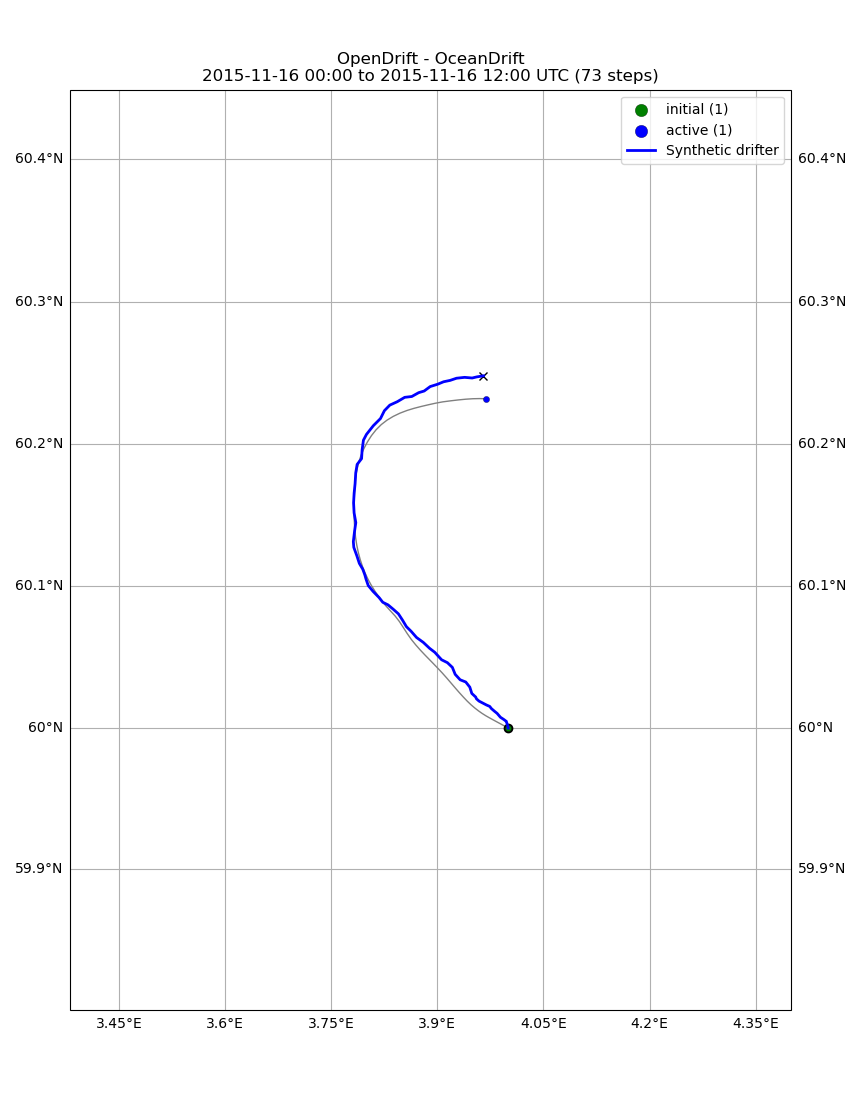
(<GeoAxes: title={'center': 'OpenDrift - OceanDrift\n2015-11-16 00:00 to 2015-11-16 12:00 UTC (73 steps)'}>, <Figure size 713.002x1100 with 1 Axes>)
The mean retrieved wind_drift_factor is 0.036, slichtly higher than the value 0.033 used for the simulation. The difference is due to the “noise” added by horizontal diffusion. Note that the retieved wind_drift_factor is linked to the wind and current used for the retrieval, other forcing datasets will yeld different value of the wind_drift_factor.
print(wind_drift_factor.mean())

plt.hist(wind_drift_factor, label='Retrieved wind_drift_factor')
plt.axvline(x=0.033, label='Actual wind_drift_factor of 0.033', color='k')
plt.axvline(x=wind_drift_factor.mean(), label='Mean retieved wind_drift_factor of %.3f' % wind_drift_factor.mean(), color='r')
plt.ylabel('Number')
plt.xlabel('Wind drift factor  [fraction]')
plt.legend(loc='lower left')
plt.show()
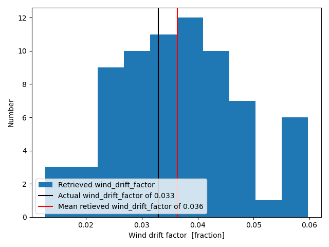
0.03639823255600984
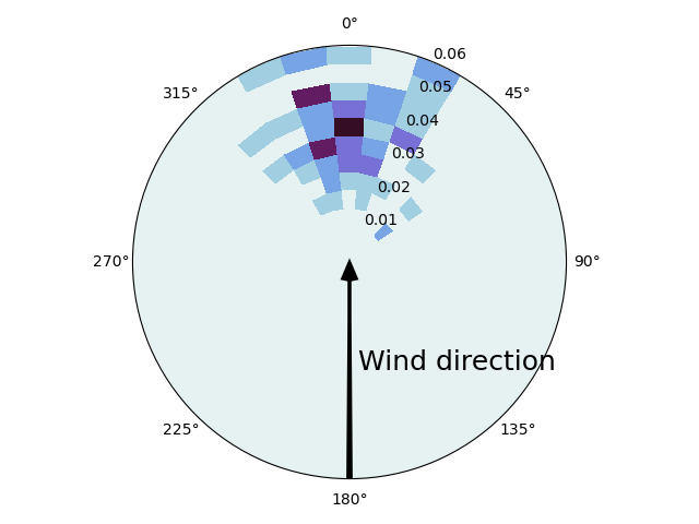
A polar 2D histogram showing also the azimuth offset direction of the retrieved wind drift factor. See Sutherland et al. (2020), https://doi.org/10.1175/JTECH-D-20-0013.1
wmax = wind_drift_factor.max()
wbins = np.arange(0, wmax+.005, .005)
abins = np.linspace(-180, 180, 30)
hist, _, _ = np.histogram2d(azimuth, wind_drift_factor, bins=(abins, wbins))
A, W = np.meshgrid(abins, wbins)
fig, ax = plt.subplots(subplot_kw=dict(projection='polar'))
ax.set_theta_zero_location('N', offset=0)
ax.set_theta_direction(-1)
pc = ax.pcolormesh(np.radians(A), W, hist.T, cmap=cmocean.cm.dense)
plt.arrow(np.pi, wmax, 0, -wmax, width=.015, facecolor='k', zorder=100,
          head_width=.8, lw=2, head_length=.005, length_includes_head=True)
plt.text(np.pi, wmax*.5, ' Wind direction', fontsize=18)
plt.grid()
plt.show()
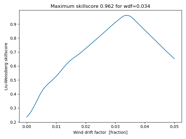
Alternative method, using skillscore
Here we calculate trajectories for a range of wind_drift_factors, and calculate the Liu-Weissberg skillscore for each. The optimized wind_drift_factor corresponds to the maximum skillscore.
o = OceanDrift(loglevel=50)
o.add_readers_from_list([tdf +
    '16Nov2015_NorKyst_z_surface/norkyst800_subset_16Nov2015.nc',
    tdf + '16Nov2015_NorKyst_z_surface/arome_subset_16Nov2015.nc'], lazy=False)
Calulating trajectories for 100 different wind_drift_factors between 0 and 0.05
wdf = np.linspace(0.0, 0.05, 100)
o.seed_elements(lon=4, lat=60, time=ot.start_time,
                wind_drift_factor=wdf, number=len(wdf))
o.run(duration=timedelta(hours=12), time_step=600)
o.plot(linecolor='wind_drift_factor', drifter=drifter)
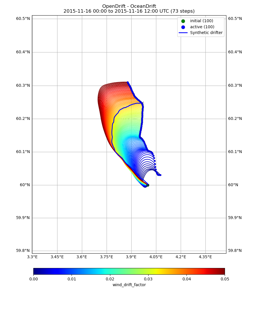
(<GeoAxes: title={'center': 'OpenDrift - OceanDrift\n2015-11-16 00:00 to 2015-11-16 12:00 UTC (73 steps)'}>, <Figure size 817.995x1100 with 2 Axes>)
Using TrajAn to calculate skillscore
skillscore = o.result.traj.skill(ot.result, tolerance_threshold=1)
Plotting and finding the wind_drift_factor which maximises the skillscore
ind = skillscore.argmax()
plt.plot(wdf, skillscore)
plt.xlabel('Wind drift factor  [fraction]')
plt.ylabel('Liu-Weissberg skillscore')
plt.title('Maximum skillscore %.3f for wdf=%.3f' % (skillscore[ind], wdf[ind]))
plt.show()
/opt/conda/envs/opendrift/lib/python3.14/site-packages/xarray/core/dataarray.py:6439: FutureWarning: Behaviour of argmin/argmax with neither dim nor axis argument will change to return a dict of indices of each dimension. To get a single, flat index, please use np.argmin(da.data) or np.argmax(da.data) instead of da.argmin() or da.argmax().
  result = self.variable.argmax(dim, axis, keep_attrs, skipna)
We see that using skillscore from the full trajectories gives a better estimate than calculating the average of the wind_drift_factor from one position to the next (i.e. polar histogram above). This is even more clear if increasing the diffusivity (i.e. noise) above from 10 m2/s to 200 m2/s: The histogram method then gives 0.071, which is much to high (true is 0.033), and the histogram is noisy. The skillscore method is still robust, and gives a wind_drift_factor of 0.034, only slightly too high.
Total running time of the script: (0 minutes 32.409 seconds)