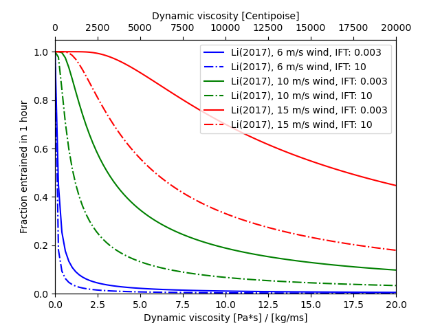
Oil entrainment rate

import numpy as np
import matplotlib.pyplot as plt
from opendrift.models.physics_methods import oil_wave_entrainment_rate_li2017

Viscosities from 0 to 20 Pa*s / kg/ms

vis = np.linspace(0, 20, 100)

colors = ['b', 'g', 'r']
lstyles = ['-', '-.']

Calculating and plotting the entrainment rate as function of viscosity for 3 wind speeds

fig, ax = plt.subplots()
for wind, color in zip([6, 10, 15], colors):

    # Entrainment rate from Li (2017)
    for ift, ls in zip([.003, 10], lstyles):
        r = oil_wave_entrainment_rate_li2017(
                dynamic_viscosity=vis, oil_density=950, interfacial_tension=ift,
                wind_speed=wind)
        # from instantaneous rate (s-1) we calculate the probability of entrainment within one hour:
        p1h = 1-np.exp(-3600*r)
        ax.plot(vis, p1h, color+ls, label='Li(2017), %s m/s wind, IFT: %s' % (wind, ift))

plt.legend()
ax.set_xlim(vis.min(), vis.max())
ax.set_ylim(0, 1.05)

# Make second x-axis showing viscosity in Centipoise
ax2 = ax.twiny()
x1, x2 = ax.get_xlim()
ax2.set_xlim(1000*x1, 1000*x2)
ax2.figure.canvas.draw()
ax2.set_xlabel('Dynamic viscosity [Centipoise]')

ax.set_ylabel('Fraction entrained in 1 hour')
ax.set_xlabel('Dynamic viscosity [Pa*s] / [kg/ms]')

plt.show()