Tutorial
OpenDrift does come with a basic graphical user interface, but the most flexible and powerful way to operate the model is through a set of Python commands. This requires only basic knowledge of Python.
The best way to get familiar with OpenDrift is to run and examine/edit the example-scripts located in the examples folder (also shown in the gallery). The main steps involved are explained below.
1. Import a specific model for the relevant application
The first step is to decide which model to use, based on your application. All available models are stored in the subfolder models. The .py files in this folder are Python “modules” containing a class which is a subclass (specialisation) of the generic class OpenDriftSimulation.
The most basic model, OceanDrift, is suitable for passive tracers (substances with no properties except for position, flowing with the ocean current) or objects at the ocean surface which may be subject to an additional wind drag. OceanDrift may be imported with the command:
from opendrift.models.oceandrift import OceanDrift
For Search and Rescue applications, the Leeway model (class) may be imported with the command:
from opendrift.models.leeway import Leeway
For oil drift applications, import the OpenOil model by the command:
from opendrift.models.openoil import OpenOil
A simulation instance (object) is created by calling the imported class:
o = OpenOil(loglevel=0)
The argument loglevel is optional, and 0 (debug mode, default) means that a lot of diagnostic information is displayed to the terminal during the run. This may be useful if something goes wrong. Use a value of 20 to get only a minimum of information, or a value of 50 for no output at all.
OpenOil uses the element type Oil (subclass of LagrangianArray), which defines some properties specific to oil (e.g. density, viscosity…). The element class may be defined in the same module/file as the trajectory model class, as in this case, or imported from the various element types in the subfolder opendrift.elements, for possible re-use by other models.
Any model contains at least the function update() which is called at each step of the model run to update the positions and properties of particles (added when seeding, see below) using environmental data (wind, current, temperature…) provided by some readers (below). A specific model implementation does not need to worry about map projections, vector orientations, how data are obtained, etc - it will focus on the advection/physical/chemical processes only.
With OpenDrift it is fairly easy to make your own model/class by simply defining element properties and an update function to describe the desired advection and other processes.
2. Adding Readers
Readers are independent Python objects which provide the variables (e.g. current, wind, temperature…) needed by the model to update particle properties. Readers normally read from a file (hence the name) or from a remote URL, or use some analytical function such as this idealistic eddy.
Different reader classes exist for different file types. E.g. for data following the NetCDF CF-convention, use the following class:
from opendrift.readers import reader_netCDF_CF_generic
A Reader instance may then be created to obtain data from a local file:
reader_norkyst = reader_netCDF_CF_generic.Reader('norkyst800_16Nov2015.nc')
To generate a reader for data on a Thredds server (here the same reader class may be used, as files are still CF-compliant):
reader_norkyst = reader_netCDF_CF_generic.Reader(
    'https://thredds.met.no/thredds/dodsC/sea/norkyst800m/1h/aggregate_be')
The reader can be inspected with:
print(reader_norkyst)
===========================
Reader: https://thredds.met.no/thredds/dodsC/sea/norkyst800m/1h/aggregate_be
Projection:
  +proj=stere +ellps=WGS84 +lat_0=90.0 +lat_ts=60.0 +x_0=3192800 +y_0=1784000 +lon_0=70
Coverage: [m]
  xmin: 0.000000   xmax: 2080800.000000   step: 800   numx: 2602
  ymin: 0.000000   ymax: 720800.000000   step: 800   numy: 902
  Corners (lon, lat):
    ( -1.58,  58.50)  ( 23.71,  75.32)
    (  9.19,  55.91)  ( 38.06,  70.03)
Vertical levels [m]:
  [-0.0 -3.0 -10.0 -15.0 -25.0 -50.0 -75.0 -100.0 -150.0 -200.0 -250.0
 -300.0 -500.0 -1000.0 -2000.0 -3000.0]
Available time range:
  start: 2017-02-20 00:00:00   end: 2019-09-08 18:00:00   step: 1:00:00
    22339 times (3120 missing)
Variables:
  y_wind
  sea_water_temperature
  upward_sea_water_velocity
  eastward_sea_water_velocity
  salinity_vertical_diffusion_coefficient
  y_sea_water_velocity
  longitude
  latitude
  sea_floor_depth_below_sea_level
  northward_sea_water_velocity
  sea_water_salinity
  x_sea_water_velocity
  time
  forecast_reference_time
  sea_surface_elevation
  x_wind

===========================
The suitability of a file or URL may also be tested from the Linux/DOS command line:
$ ./scripts/readerinfo.py <filename/URL>
Adding the option -p to the above command will also plot the geographical coverage. From Python the same plot can be obtained with the command reader_norkyst.plot()
The coverage of the NorKyst ocean model on the met.no Thredds server may e.g. be plotted with the following command:
readerinfo.py https://thredds.met.no/thredds/dodsC/sea/norkyst800m/1h/aggregate_be -p

The variables (e.g. wind, current…) required by a specific model are given in the list “required_variables” in the model class implementation, and may be listed by:
>>> from pprint import pprint
>>> pprint(OpenOil.required_variables)
   {'land_binary_mask': {'fallback': 0},
    'ocean_vertical_diffusivity': {'fallback': 0.02,
                                   'important': False,
                                   'profiles': True},
    'sea_ice_area_fraction': {'fallback': 0, 'important': False},
    'sea_ice_x_velocity': {'fallback': 0, 'important': False},
    'sea_ice_y_velocity': {'fallback': 0, 'important': False},
    'sea_surface_wave_mean_period_from_variance_spectral_density_second_frequency_moment': {'fallback': 0,
                                                                                            'important': False},
    'sea_surface_wave_period_at_variance_spectral_density_maximum': {'fallback': 0,
                                                                     'important': False},
    'sea_surface_wave_significant_height': {'fallback': 0, 'important': False},
    'sea_surface_wave_stokes_drift_x_velocity': {'fallback': 0,
                                                 'important': False},
    'sea_surface_wave_stokes_drift_y_velocity': {'fallback': 0,
                                                 'important': False},
    'sea_water_salinity': {'fallback': 34, 'profiles': True},
    'sea_water_temperature': {'fallback': 10, 'profiles': True},
    'upward_sea_water_velocity': {'fallback': 0, 'important': False},
    'x_sea_water_velocity': {'fallback': None},
    'x_wind': {'fallback': None},
    'y_sea_water_velocity': {'fallback': None},
    'y_wind': {'fallback': None}}
Variable names follow the CF-convention, ensuring that any reader may be used by any model, although developed independently. It is necessary to add readers for all required variables, unless they have been given a fallback (default) value which is not None. In the above example, it is only strictly necessary to provide readers for wind and current. The fallback values will be used for elements which move out of the coverage of a reader in space or time, if there is no other readers which provides the given variable. Variables where important is set to False will only be obtained from readers which are already available, new lazy readers will not be initialized if these are missing. Most applications will need a landmask, for stranding towards a coastline. The default is to use the global GSHHG database landmask, unless explicitly disabled with:
o.set_config('general:use_auto_landmask', False)
After Readers are created, they must be added to the model instance:
o.add_reader([reader_landmask, reader_norkyst, reader_nordic])
The order will decide if several readers provide the same variable. In the above example, current will be obtained from the Reader reader_norkyst whenever possible, or else from the Reader reader_nordic. The landmask will be taken from the landmask reader since this is listed first, even if the other readers would also contain a landmask (e.g. a coarse raster used by the ocean model).
When later running a simulation, the readers will first read data from file/URL, before interpolating onto the element positions. The default horizontal interpolation method is ‘LinearNDFast’, which interpolates/fill holes (e.g. islands in a coarse ocean model may appears as a large square of no values) and extrapolates towards the (GSHHG) coastline.
Readers also take care of reprojecting all data from their native map projection to a common projection, which is generally necessary as different readers may have different projection. This allows OpenDrift to use raw output from ocean/wave/atmosphere models, without the need to preprocess large amounts of data. Vectors (wind, current) are also rotated to the common calculation projection. By default, the common projection is taken from the first added reader, so that data from this reader must not be reprojected/rotated.
In addition to providing variables interpolated to the element positions, readers will also provide vertical profiles (e.g. from a 3D ocean model) at all positions for variables where profiles is True in the variable listing above. Profiles are here obtained for salinity, temperature and diffusivity, as these are used for the vertical mixing algorithm. See Vertical mixing for a demonstration.
2.1 Lazy Readers
For an operational setup, it is convenient to have a long priority list of available readers/sources, to be sure that the desired location and time is covered by forcing data. However, initialising all readers before the simulation starts may then take some time, especially if the list of readers include some slow or potentially hanging Thredds servers.
The concept of Lazy Readers allows to delay the initialisation of readers until they are actually needed. This minimises statup time, and decreases the risk of hanging. Readers are by default Lazy if they are initiated with the methods add_readers_from_list(<list_of_reader_filenames/URLs>) or add_readers_from_file(<file_with_lines of_reader_filenames/URLs>), e.g.:
o.add_readers_from_list(['somelocalfile.nc',
       'https://thredds.met.no/thredds/dodsC/sea/norkyst800m/1h/aggregate_be',
       'https://thredds.met.no/thredds/dodsC/sea/nordic4km/zdepths1h/aggregate_be'])
Printing the simulation object then shows that these have been added as lazy readers. Since initialisation of these have been delayed, we do not yet know whether they cover the required variables, but this will be checked whenever necessary during the upcoming simulation:
print(o)
===========================
Model:      OceanDrift     (OpenDrift version 1.0.5)
    0 active PassiveTracer particles  (0 deactivated, 0 scheduled)
Projection: +proj=latlong
-------------------
Environment variables:
  -----
Readers not added for the following variables:
  land_binary_mask
  x_sea_water_velocity
  x_wind
  y_sea_water_velocity
  y_wind
---
Lazy readers:
  LazyReader: somelocalfile.nc
  LazyReader: https://thredds.met.no/thredds/dodsC/sea/norkyst800m/1h/aggregate_be
  LazyReader: https://thredds.met.no/thredds/dodsC/sea/nordic4km/zdepths1h/aggregate_be
===========================
If somelocalfile.nc contains the required variables for the element positions throughout the simulation, the Thredds-readers will never be initialised, thus saving time.
If you want readers to be intialised immediately, you may provide the keyword lazy=False to add_readers_from_list() or add_readers_from_file().
These methods are robust regarding nonexisting files or URLs, which will then be marked as “Discarded readers” during the simulation.
3. Seeding elements
Before starting a model run, some elements must be seeded (released). The simplest case is to seed a single element at a given position and time:
o.seed_elements(lon=4.3, lat=60, time=datetime(2016,2,25,18,0,0))
The time may be defined explicitly as in the above example, or one may e.g. use the starting time of one of the available readers (e.g. time=reader_norkyst.start_time). To seed 100 elements within a radius of 1000 m:
o.seed_elements(lon=4.3, lat=60, number=100, radius=1000,
                time=reader_norkyst.start_time)
Note that the radius is not an absolute boundary within which elements will be seeded, but one standard deviation of a normal distribution in space. Thus about 68% of elements will be seeded within this radius, with more elements near the center.
By default, elements are seeded at the surface (z=0), but the depth may be given as a negative scalar (same for all elements), or as a vector of the same length as the number of elements. Elements may also be seeded at the seafloor by specifying z='seafloor', however, this requires that a reader providing the variable sea_floor_depth_below_sea_level has been already been added. It is also possible to seed elements a given height above seafloor, e.g. z='seafloor+50' to seed elements 50m above seafloor.
All seeded elements will get the default values of any properties as defined in the model implementation, or the properties may be specified (overridden) with a name-value pair:
o.seed_elements(lon=4.3, lat=60, number=100, radius=1000,
                density=900, time=reader_norkyst.start_time)
This will give all 100 oil elements (if o is an OpenOil instance) a density of 900 kg/m3, instead of the default value of 880 kg/m3. To assign unique values to each element, the properties may be given as an array with length equal the number of elements:
from numpy import random
o.seed_elements(lon=4.3, lat=60, number=100, radius=1000,
                density=random.uniform(880, 920, 100),
                time=reader_norkyst.start_time)
The properties of the seeded elements may be displayed with:
o.elements_scheduled
Elements may be seeded along a line (or cone) between two points by using the method seed_cone. Lon and lat must then be two element arrays, indicating start and end points. An uncertainty radius may also be given as a two element array, thus tracing out a cone (where a line is a special case with same radius at both ends):
o.seed_cone(lon=[4, 4.8], lat=[60, 61], number=1000, radius=[0, 5000],
            time=reader_norkyst.start_time)
If time is also given as a two element list (of datetime objects), elements are seeded linearly in time (here over a 5 hour interval):
o.seed_cone(lon=[4, 4.8], lat=[60, 61], number=1000, radius=[0, 5000],
            time=[norkyst.start_time, norkyst.start_time+timedelta(hours=5)])
Specific OpenDrift models may have additional seed-functions. E.g. opendrift.models.openoil contains a function (seed_from_gml) to seed oil elements within contours from satellite detected oil slicks read from a GML-file. The Leeway model overloads the generic seed_elements function since it needs to read some object properties from a text-file.
The seed functions may also be called repeatedly before starting the simulation, try Grid time for an example of this.
Run the script Seed demonstration for a demonstration of various ways to seed elements.
4. Configuration
OpenDrift allows for configuration of the model using the package ConfigObj. The properties which can be configured can be listed by the command:
o.list_configspec()
Parameters may be set with commands like:
o.set_config('drift:advection_scheme', 'runge-kutta')
This example specifies that the Runge-Kutta propagation scheme shall be used for the run, instead of the default Euler-scheme.
The following command specifies that the elements at the ocean surface shall drift with 2 % of the wind speed (in addition to the current):
o.set_config('seed:wind_drift_factor', .02)
The configuration value is retrieved by:
wind_drift_factor = o.get_config('seed:wind_drift_factor')
See the example-files for more examples of configuration.
5. Running the model
After initialisation, adding readers and seeding elements, a model run (simulation) can be started by calling the function run:
o.run()
The simulation will start at the time of the first seeded element, and continue until the end of any of the added readers. The default time step is one hour (3600 seconds). The calculation time step may be specified with the parameter time_step, in seconds, or as a datetime.timedelta object:
o.run(time_step=900)
which is equivalent to:
from datetime import timedelta
o.run(time_step=timedelta(minutes=15))
The duration of the simulation may be specified by providing one (and only one) of the following parameters:
steps[integer] The number of calculation steps
duration[datetime.timedelta] The length of the simulation
end_time[datetime.datetime] The end time of the simulation
The output may be saved to a file, if specifying outfile=<filename>.
Currently only one output format is supported: the NetCDF CF convention on Trajectory data.
A sample output NetCDF file is available here.
It is possible to make “writers” for other output formats, and these must be stored in the subfolder export.
By default, all element properties (position (lon/lat/z), density etc) and all environment variables (current, wind etc) are saved to the file, and are stored in an array o.history in memory for plotting and analysis. There are two ways to reduce the memory consumption and file size:
save only a subset of the variables/parameters by providing
export_variables[list of strings]save data only at a specified time interval by providing
time_step_output[seconds, or timedelta]. The output time step must be larger or equal to the calculation time step, and must be an integer multiple of this.
The following command will run a simulation from the first seeding time until the end of the reader_norkyst reader (current data) with a calculation time step of 15 minutes, but output (saved) only every hour. The properties ‘density’ and ‘water_content’ are saved to the file ‘openoil.nc’ (in addition to the obligatory element properties ‘lon’ and ‘lat’, and the internal parameters ‘ID’ and ‘status’):
o.run(end_time=reader_norkyst.end_time, time_step=900,
      time_step_output=3600, outfile='openoil.nc',
      export_variables=['density', 'water_content'])
The saved output may later be imported with the commands:
o = OpenOil()
o.io_import_file(<filename>)
During a model run, the following actions are performed repeatedly at the given calculation time step:
Readers are called successively to retrieve all required environment variables, and interpolate onto the element positions.
Element properties and positions are updated by the model specific function
update()Elements are deactivated if any required_variables are missing (and there is no fallback_value), or by any other reason as specified in the relevant
update()function (e.g. stranding towards coast, or “evaporated”).
The run continues until one of the following conditions are met:
All elements have been deactivated
The specified end time has been reached (as given by
end_time,durationorsteps)Anything crashes during the simulation, for any given reason (which is displayed to the terminal)
6. Plotting and analysing the results
After the run (or after importing from a file), the status can be inspected:
print(o)

===========================
Model:      OpenOil
    83 active Oil particles  (17 deactivated)
Projection: +proj=stere +lat_0=90 +lon_0=70 +lat_ts=60 +units=m +a=6.371e+06 +e=0 +no_defs
-------------------
Environment variables:
  -----
  x_sea_water_velocity
  y_sea_water_velocity
     1) https://thredds.met.no/thredds/dodsC/sea/norkyst800m/1h/aggregate_be
  -----
  x_wind
  y_wind
     1) https://thredds.met.no/thredds/dodsC/arome25/arome_metcoop_default2_5km_latest.nc
  -----
  land_binary_mask
     1) global_landmask
Time:
    Start: 2015-03-04 06:00:00
    Present: 2015-03-12 14:00:00
    Iterations: 200
Time spent:
    Fetching environment data: 0:00:15.250431
    Updating elements: 0:00:00.268629
===========================
A map showing the trajectories is plotted with the command o.plot()
The trajectories may be colored by any of the element properties by giving the keyword linecolor to the plot function, e.g.:
o.plot(linecolor='z')
which will color lines according to depth (z):
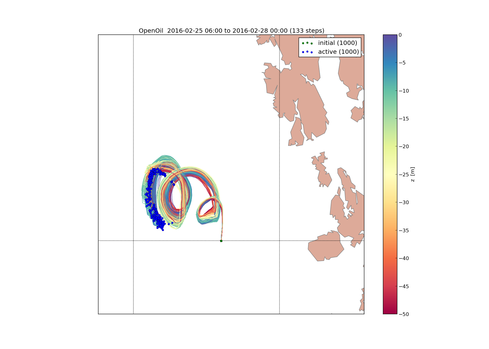
Green stars mark initial (seeding) positions, and blue elements are still active at end of simulation.
A variable field from any of the readers may be used as background to the plot by providing the variable name as the keyword string background. Vector fields (winds, current) may also be plotted by giving the x- and y-components in a two element list:
o.plot(background=['x_sea_water_velocity', 'y_sea_water_velocity'])
This may be useful for visualising where the model (reader) eventually may be missing data (white areas on the plot below). Note that the “holes” will be filled/interpolated during the simulation, with the default interpolation method (‘LinearNDFast’, see above). Contourlines are plotted instead of background color if parameter ‘contourlines’ is set to True or to a list of values for the contour levels.

o.animation() will show an animation of the last run.
An animation comparing two runs is obtained by:
o.animation(compare=o2, legend=['Current + 3 % wind drift', 'Current only'])
where o2 is another simulation object (or filename of saved simulation). The legend items correspond to the first (o) and second (o2) simulations. The two runs must have identical time steps and start time.
The animation may be saved to file if providing the keyword filename. Supported output is animated GIF (if file suffix is .gif, and if imagemagick is available) or otherwise mp4 (file suffix .mp4). For mp4 you might need to install ffmpeg or mencoder if not already available on your system.
The quality of mp4-files is quite low with older versions of Matplotlib, as bitrate may not be set manually. With newer versions of Matplotlib, the animate function might however need some updates to work properly (please report any errors).
When exporting animation to mp4, an additional parameter fps may be provided to specify the number of frames per seconds (speed of animation), default is 20 frames/second.
Specific models may define specific plotting functions. One example is OpenOil.plot_oil_budget() which plots the oil mass budget of a simulation.
The examples Cod egg and Oil vertical mixing demonstrate the function plot_vertical_distribution() to show a histogram of the element depths, with an interactive time slider.
See the gallery for some examples of output figures and animations.