Note
Go to the end to download the full example code.
Double gyre, advection
Illustrating the difference between Euler and Runge-Kutta propagation schemes, using an idealised (analytical) eddy current field.
Double gyre current field from https://shaddenlab.berkeley.edu/uploads/LCS-tutorial/examples.html
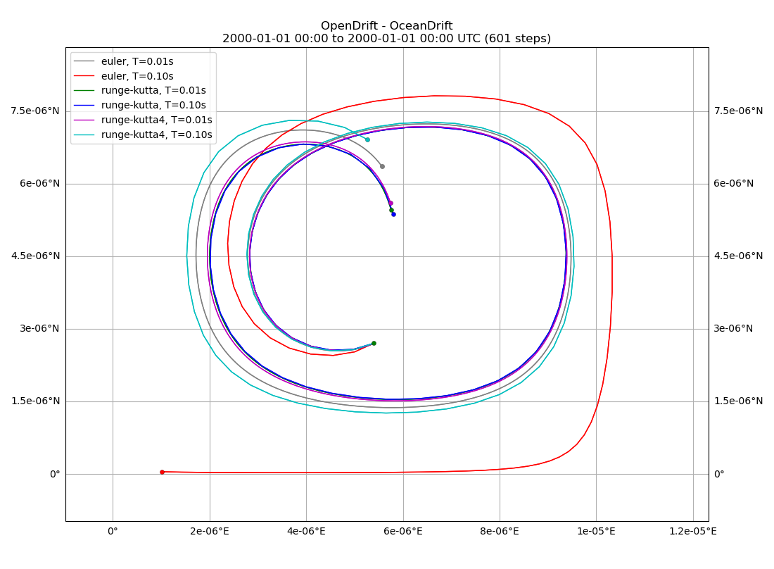
euler, T=0.01s
euler, T=0.10s
runge-kutta, T=0.01s
runge-kutta, T=0.10s
runge-kutta4, T=0.01s
runge-kutta4, T=0.10s

(<GeoAxes: title={'center': 'OpenDrift - OceanDrift\n2000-01-01 00:00 to 2000-01-01 00:00 UTC (601 steps)'}>, <Figure size 1100x808.707 with 1 Axes>)
import numpy as np
from datetime import datetime, timedelta

from opendrift.readers import reader_double_gyre
from opendrift.models.oceandrift import OceanDrift

double_gyre = reader_double_gyre.Reader(epsilon=.25, omega=0.628, A=0.25)
duration=timedelta(seconds=6)
x = [.6]
y = [.3]
lon, lat = double_gyre.xy2lonlat(x, y)

runs = []
leg = []
i = 0
for scheme in ['euler', 'runge-kutta', 'runge-kutta4']:
    for time_step  in [0.01, 0.1]:
        leg.append(scheme + ', T=%.2fs' % time_step)
        print(leg[-1])
        o = OceanDrift(loglevel=50)
        o.set_config('environment:fallback:land_binary_mask', 0)
        o.set_config('drift:advection_scheme', scheme)
        o.add_reader(double_gyre)
        o.seed_elements(lon, lat, time=double_gyre.initial_time)
        o.run(duration=duration, time_step=time_step)
        runs.append(o)
        i = i + 1

runs[0].plot(compare=runs[1:], legend=leg, buffer=0.000001, hide_landmask=True)
Total running time of the script: (1 minutes 1.070 seconds)