Examples of leveraging xarray in combination with trajan to analyze OMB data

import matplotlib.pyplot as plt
from pathlib import Path
from trajan.readers.omb import read_omb_csv
from trajan.plot.spectra import plot_trajan_spectra
import coloredlogs
import datetime

# a few helper functions


def print_head(filename, nlines=3):
    """Print the first nlines of filename"""
    print("----------")
    print(f"head,{nlines} of {filename}")
    print("")
    with open(filename) as input_file:
        head = [next(input_file) for _ in range(nlines)]
    for line in head:
        print(line, end="")
    print("----------")

# adjust the level of information printed

coloredlogs.install(level='error')
# coloredlogs.install(level='debug')

# We start by preparing some example data to work with

# generate a trajan dataset
path_to_test_data = Path.cwd().parent / "tests" / "test_data" / "csv" / "omb3.csv"
xr_buoys = read_omb_csv(path_to_test_data)

# list all the buoys in the dataset

list_buoys = list(xr_buoys.trajectory.data)
print(f"{list_buoys = }")

list_buoys = [np.str_('drifter_1'), np.str_('drifter_2'), np.str_('drifter_3')]

# some users prefer to receive CSV files to perform their analysis: dump all trajectories as CSV

# all positions to CSV, 1 CSV per buoy
for crrt_buoy in list_buoys:
    crrt_xr = xr_buoys.sel(trajectory=crrt_buoy)
    crrt_xr_gps = crrt_xr.swap_dims({'obs': 'time'})[["lat", "lon"]]
    crrt_xr_gps = crrt_xr_gps.dropna(dim='time')
    crrt_xr_gps.to_dataframe().to_csv(f"{crrt_buoy}_gps.csv")

print_head("drifter_1_gps.csv")

----------
head,3 of drifter_1_gps.csv

time,lat,lon,trajectory
2022-06-15 09:30:27,79.4024501,3.0311076,drifter_1
2022-06-15 10:00:41,79.3992077,3.0430603,drifter_1
----------

# similarly, some users prefer to receive CSV files for the wave information to perform their analysis

# scalar data are easy to dump: the following creates files with
# all wave statistics to CSV, 1 file per buoy
for crrt_buoy in list_buoys:
    crrt_xr = xr_buoys.sel(trajectory=crrt_buoy)
    crrt_xr_wave_statistics = crrt_xr.swap_dims({"obs_waves_imu": "time_waves_imu"})[["pcutoff", "pHs0", "pT02", "pT24", "Hs0", "T02", "T24"]].rename({"time_waves_imu": "time"}).dropna(dim="time")
    crrt_xr_wave_statistics.to_dataframe().to_csv(f"{crrt_buoy}_wavestats.csv")

print_head("drifter_1_wavestats.csv")

# for spectra, we need to get the frequencies first and to label things
# all spectra to CSV, 1 file per buoy, 1 frequency per columns
for crrt_buoy in list_buoys:
    crrt_xr = xr_buoys.sel(trajectory=crrt_buoy)
    # the how="all" is very important: since in the processed spectrum the "invalid / high noise" bins are set to NaN, we must only throw away the wave spectra for which all
    # bins are nan, but we must keep the spectra for which a few low frequency bins are nan.
    # if you want a CSV without any NaN, you can use "elevation_energy_spectrum" instead of "processed_elevation_energy_spectrum" to use the spectra with all bins, including
    # the bins that are dominated by low frequency noise
    crrt_xr_wave_spectra = crrt_xr.swap_dims({"obs_waves_imu": "time_waves_imu"})[["processed_elevation_energy_spectrum"]].rename({"time_waves_imu": "time"}).dropna(dim="time", how="all")

    list_frequencies = list(crrt_xr_wave_spectra.frequencies_waves_imu.data)

    for crrt_ind, crrt_freq in enumerate(list_frequencies):
        crrt_xr_wave_spectra[f"f={crrt_freq}"] = (['time'],  crrt_xr_wave_spectra["processed_elevation_energy_spectrum"][:, crrt_ind].data)

    crrt_xr_wave_spectra = crrt_xr_wave_spectra.drop_vars("processed_elevation_energy_spectrum").drop_dims("frequencies_waves_imu")
    crrt_xr_wave_spectra.to_dataframe().to_csv(f"{crrt_buoy}_wavespectra.csv", na_rep="NaN")

print_head("drifter_1_wavespectra.csv")

----------
head,3 of drifter_1_wavestats.csv

time,pcutoff,pHs0,pT02,pT24,Hs0,T02,T24,trajectory
2022-06-15 09:22:17,6.0,0.01314965113641037,10.96823590753681,10.31552944794857,0.019197048619389534,13.503824739884486,11.430906656065092,drifter_1
2022-06-15 12:21:39,4.0,0.025573064649650458,11.612432009831267,11.177067212654027,0.028518375009298325,12.404869941212194,11.482618108622855,drifter_1
----------
----------
head,3 of drifter_1_wavespectra.csv

time,trajectory,f=0.0439453125,f=0.048828125,f=0.0537109375,f=0.05859375,f=0.0634765625,f=0.068359375,f=0.0732421875,f=0.078125,f=0.0830078125,f=0.087890625,f=0.0927734375,f=0.09765625,f=0.1025390625,f=0.107421875,f=0.1123046875,f=0.1171875,f=0.1220703125,f=0.126953125,f=0.1318359375,f=0.13671875,f=0.1416015625,f=0.146484375,f=0.1513671875,f=0.15625,f=0.1611328125,f=0.166015625,f=0.1708984375,f=0.17578125,f=0.1806640625,f=0.185546875,f=0.1904296875,f=0.1953125,f=0.2001953125,f=0.205078125,f=0.2099609375,f=0.21484375,f=0.2197265625,f=0.224609375,f=0.2294921875,f=0.234375,f=0.2392578125,f=0.244140625,f=0.2490234375,f=0.25390625,f=0.2587890625,f=0.263671875,f=0.2685546875,f=0.2734375,f=0.2783203125,f=0.283203125,f=0.2880859375,f=0.29296875,f=0.2978515625,f=0.302734375,f=0.3076171875
2022-06-15 09:22:17,drifter_1,NaN,NaN,NaN,NaN,NaN,NaN,0.00018836664667848252,0.0002536176619217721,0.00037407416146983946,0.0005160847238443518,0.0004775387927092086,0.00021705670077672262,0.00010799651982006195,8.118276215051368e-05,4.540140398252498e-05,1.6798184104757763e-05,8.735491892326276e-06,3.37320075174786e-06,2.3330519862623306e-06,1.637119173799135e-06,9.367502273162999e-07,8.794225974447227e-07,1.3622546348014245e-06,1.1559618375322706e-06,8.91298176848868e-07,8.619055226622198e-07,7.407467362281772e-07,7.153909256258964e-07,5.021764310584239e-07,5.101399987499334e-07,3.790938595016995e-07,3.743723938561384e-07,4.259018780147452e-07,4.436881227507446e-07,3.254183285148178e-07,3.9926199856911364e-07,2.3838854957946684e-07,1.4369698321522603e-07,2.0935468879394994e-07,1.5709519793897106e-07,2.403222134246955e-07,2.4403126024964503e-07,2.1483289035046126e-07,1.398516460740184e-07,1.0131942148225752e-07,8.467447363268691e-08,9.02962557337194e-08,6.814839567432175e-08,6.539515091041584e-08,9.145836305355132e-08,8.201608058798856e-08,5.769733271205716e-08,4.225047292134682e-08,6.343451709810667e-08,7.882926596568082e-08
2022-06-15 12:21:39,drifter_1,NaN,NaN,NaN,NaN,0.00022508918710088845,0.0003262487709032901,0.000640393529648558,0.0012896659656748508,0.0015856712651376335,0.002136675269053399,0.001439104532161295,0.0005376073753482228,0.0002023107894620826,5.0261273257044134e-05,1.0111549107485083e-05,4.982023062740557e-06,3.984113427413131e-06,2.514583310003887e-06,3.324528737718034e-06,2.2681116369240297e-06,2.737070959127396e-06,2.6668863062799185e-06,2.6678820406403294e-06,2.0469425719842334e-06,1.1231732000184705e-06,1.0845480786331816e-06,1.595888260841469e-06,1.3128225931972327e-06,1.0053121549167107e-06,9.135238249013721e-07,6.279699394278049e-07,6.631935969815e-07,7.559105543839675e-07,5.07906187366437e-07,3.8355262676897935e-07,3.8299915143116864e-07,3.820506868776343e-07,3.468138032292902e-07,2.3619474021022772e-07,1.846156771683609e-07,2.1728887529956186e-07,2.2581795895398703e-07,1.0864608618406476e-07,1.2365255766160254e-07,1.2638907966302735e-07,9.65866503389761e-08,1.7724022269307005e-07,1.256163313766712e-07,9.283978038002852e-08,5.2448329430694313e-08,6.777727400254332e-08,8.626908578621141e-08,7.875586931394864e-08,6.655693116093259e-08,5.103979369513389e-08
----------

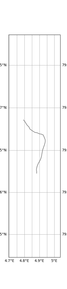
# it is easy to look into one single trajectory and select a time slice:
# (note that, for trajectories coming from buoys that have "real world", buoy dependent
# sample time, one needs to select only 1 trajectory at a time, since the time axis
# has to be unique, and it will be different from buoy to buoy)

xr_specific_buoy = xr_buoys.sel(trajectory="drifter_1")

# make a restricted dataset about only the GPS data for a specific buoy, making GPS time the new dim
# this works because we now have a single buoy so there is only 1 "time" left
xr_specific_buoy_gps = xr_specific_buoy.swap_dims({'obs': 'time'})[["lat", "lon"]]

# keep only the valid GPS points: avoid the NaT that are due to time alignment in the initial nc file
xr_specific_buoy_gps = xr_specific_buoy_gps.dropna(dim='time')

# select a specific time interval
xr_specific_buoy_time_gps = xr_specific_buoy_gps.sel(time=slice("2022-06-17T10", "2022-06-18T01"))

# plot
xr_specific_buoy_time_gps.traj.plot()
plt.show()

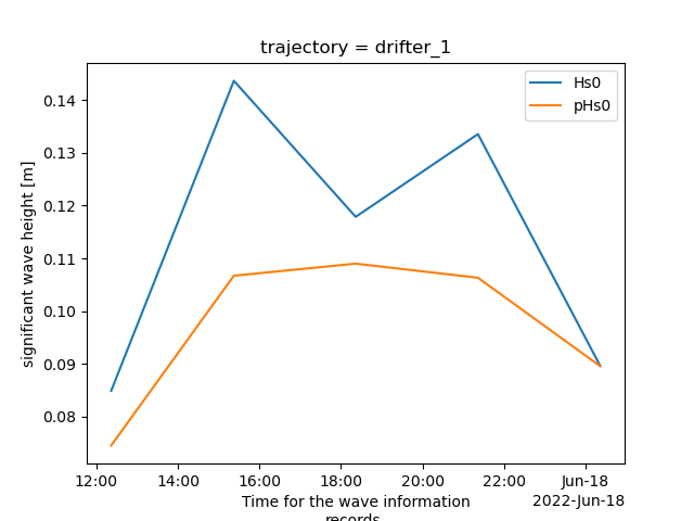
# similarly, it is easy to plot wave statistics over a given time slice:

xr_specific_buoy = xr_buoys.sel(trajectory="drifter_1")

# select the wave data for a specific buoy and make time_waves_imu the new time dim
# this works because we have only 1 buoy left, so only 1 time_waves_imu
# the how="all" is necessary to not throw away the records for which some few bins
# have been marked as nan due to the low frequency noise
xr_specific_buoy_waves = xr_specific_buoy.swap_dims({"obs_waves_imu": "time_waves_imu"})[["accel_energy_spectrum", "elevation_energy_spectrum", "processed_elevation_energy_spectrum", "pcutoff", "pHs0", "pT02", "pT24", "Hs0", "T02", "T24"]].rename({"time_waves_imu": "time"}).dropna(dim="time", how="all")

# plot, for example, swh related quantities; naturally, could use any other fields
# (except the spectra themselves that are array data)

fix, ax = plt.subplots()

xr_specific_buoy_waves_specific_time = xr_specific_buoy_waves.sel(time=slice("2022-06-17T10", "2022-06-18T01"))
for crrt_field in ["Hs0", "pHs0"]:
    xr_specific_buoy_waves_specific_time[crrt_field].plot.line(ax=ax, label=crrt_field)

plt.legend()
plt.ylabel("significant wave height [m]")
plt.show()

# to plot one or more 1D wave spectra, we have dedicated tooling:

# plot the spectra for just a few of the buoys; you could also not sel to plot the whole dataset
xr_several_buoys = xr_buoys.sel(trajectory=["drifter_1", "drifter_2"])

# tuning of start and end dates
date_start = datetime.datetime(2022, 6, 16, 0, 0, 0)
date_end = datetime.datetime(2022, 6, 18, 0, 0, 0)

plot_trajan_spectra(xr_several_buoys, tuple_date_start_end=(date_start, date_end))