Calculating gridded concentrations

import numpy as np
import matplotlib.pyplot as plt
import xarray as xr
import trajan as _

Demonstrating calculation and plotting of gridded concentrations

Importing a trajectory dataset from an oil drift simulation (OpenOil)

ds = xr.open_dataset('opv2025_subset.nc')

Make a grid covering this dataset with a horizontal resolution of 200m

grid = ds.traj.make_grid(dx=200)
print(grid)

2025-06-24 13:41:18 fv-az1280-93 trajan.accessor[2414] DEBUG Detecting trajectory dimension
2025-06-24 13:41:18 fv-az1280-93 trajan.accessor[2414] DEBUG Detected obs-dim: time, detected time-variable: time.
2025-06-24 13:41:18 fv-az1280-93 trajan.accessor[2414] DEBUG Detected structured (1D) trajectory dataset
2025-06-24 13:41:18 fv-az1280-93 trajan.traj[2414] DEBUG No grid-mapping specified, checking if coordinates are lon/lat..
<xarray.Dataset> Size: 11kB
Dimensions:    (lat: 31, lon: 38, time: 13, lat_edges: 32, lon_edges: 39)
Coordinates:
  * time       (time) datetime64[ns] 104B 2025-06-08T07:00:00 ... 2025-06-08T...
  * lat        (lat) float64 248B 59.74 59.74 59.74 59.74 ... 59.79 59.79 59.79
  * lon        (lon) float64 304B 2.187 2.19 2.194 2.197 ... 2.311 2.315 2.319
  * lat_edges  (lat_edges) float64 256B 59.74 59.74 59.74 ... 59.79 59.79 59.79
  * lon_edges  (lon_edges) float64 312B 2.185 2.189 2.192 ... 2.313 2.317 2.32
Data variables:
    cell_area  (lat, lon) float64 9kB 4.003e+04 4.003e+04 ... 3.997e+04

Calculate the concentration number of elements for this grid

ds_c = ds.traj.concentration(grid)
print(ds_c)

<xarray.Dataset> Size: 256kB
Dimensions:                    (lat: 31, lon: 38, time: 13, lat_edges: 32,
                                lon_edges: 39)
Coordinates:
  * time                       (time) datetime64[ns] 104B 2025-06-08T07:00:00...
  * lat                        (lat) float64 248B 59.74 59.74 ... 59.79 59.79
  * lon                        (lon) float64 304B 2.187 2.19 ... 2.315 2.319
  * lat_edges                  (lat_edges) float64 256B 59.74 59.74 ... 59.79
  * lon_edges                  (lon_edges) float64 312B 2.185 2.189 ... 2.32
Data variables:
    cell_area                  (lat, lon) float64 9kB 4.003e+04 ... 3.997e+04
    number                     (time, lat, lon) float64 123kB nan nan ... nan
    number_area_concentration  (time, lat, lon) float64 123kB nan nan ... nan

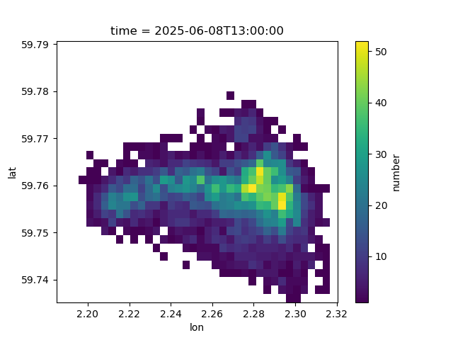
Plot the number of particles and concentration (number/area) per grid cell at a given time.

ds_c.isel(time=12).number.plot()
plt.show()

2025-06-24 13:41:19 fv-az1280-93 matplotlib.colorbar[2414] DEBUG locator: <matplotlib.ticker.AutoLocator object at 0x7f7df3e716d0>

Plot the number concentration (number/area) per grid cell at a given time. Since pixels have nearly the same size, this is nearly proportional to the previous plot.

ds_c.isel(time=12).number_area_concentration.plot()
plt.show()

2025-06-24 13:41:19 fv-az1280-93 matplotlib.colorbar[2414] DEBUG locator: <matplotlib.ticker.AutoLocator object at 0x7f7df023a9f0>

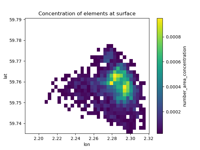
Plot the number concentration (number/area) for surface oil only (elements where z=0)

ds_surface = ds.where(ds.z==0).traj.concentration(grid)
ds_surface.isel(time=12).number_area_concentration.plot()
plt.title('Concentration of elements at surface')
plt.show()

2025-06-24 13:41:20 fv-az1280-93 trajan.accessor[2414] DEBUG Detecting trajectory dimension
2025-06-24 13:41:20 fv-az1280-93 trajan.accessor[2414] DEBUG Detected obs-dim: time, detected time-variable: time.
2025-06-24 13:41:20 fv-az1280-93 trajan.accessor[2414] DEBUG Detected structured (1D) trajectory dataset
2025-06-24 13:41:21 fv-az1280-93 matplotlib.colorbar[2414] DEBUG locator: <matplotlib.ticker.AutoLocator object at 0x7f7df023acc0>

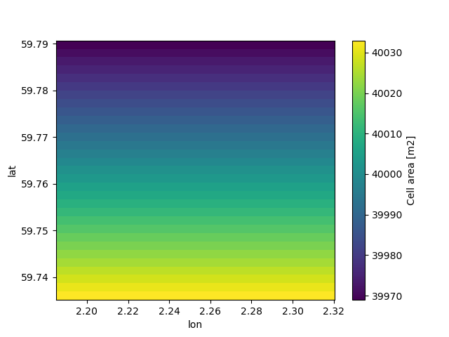
We see that the cell area decreases slightly away from equator. This is accounted for when calculating area/volume concentration.

ds_c.cell_area.plot()
plt.show()

2025-06-24 13:41:21 fv-az1280-93 matplotlib.colorbar[2414] DEBUG locator: <matplotlib.ticker.AutoLocator object at 0x7f7df3e73a40>

Making a new grid including a vertical dimension (3D), with highest resolution near the surface (z=0)

z=[-0.01, -1, -3, -5, -7.5, -10, -20, -30]
grid3d = ds.traj.make_grid(dx=400, z=z)

2025-06-24 13:41:21 fv-az1280-93 trajan.traj[2414] DEBUG No grid-mapping specified, checking if coordinates are lon/lat..

Calculate the concentration of elements for this new grid, also weighted with element property “mass_oil”

ds = ds.isel(time=12)  # Pre-selecting a single time before calculating concentrations
ds_c = ds.traj.concentration(grid3d, weights='mass_oil')

2025-06-24 13:41:21 fv-az1280-93 trajan.accessor[2414] DEBUG Detecting trajectory dimension
2025-06-24 13:41:21 fv-az1280-93 root[2414] DEBUG <xarray.Dataset> Size: 140kB
Dimensions:     (trajectory: 5000)
Coordinates:
    time        datetime64[ns] 8B 2025-06-08T13:00:00
  * trajectory  (trajectory) int32 20kB 0 1 2 3 4 5 ... 4995 4996 4997 4998 4999
Data variables:
    lat         (trajectory) float32 20kB 59.76 59.76 59.76 ... 59.76 59.76
    lon         (trajectory) float32 20kB 2.295 2.288 2.269 ... 2.29 2.255 2.248
    mass_oil    (trajectory) float32 20kB ...
    status      (trajectory) float64 40kB ...
    z           (trajectory) float32 20kB 0.0 -0.4961 0.0 ... 0.0 -17.26 -3.071
Attributes: (12/165)
    Conventions:                                                             ...
    standard_name_vocabulary:                                                ...
    featureType:                                                             ...
    title:                                                                   ...
    summary:                                                                 ...
    keywords:                                                                ...
    ...                                                                                                               ...
    geospatial_lon_resolution:                                               ...
    runtime:                                                                 ...
    geospatial_vertical_min:                                                 ...
    geospatial_vertical_max:                                                 ...
    geospatial_vertical_positive:                                            ...
    NCO:                                                                     ... has tx.dims = ('trajectory',) which is of dimension 1 but is not index; this is a bit unusual; try to parse with Traj1d or Traj2d
2025-06-24 13:41:21 fv-az1280-93 trajan.accessor[2414] DEBUG No time or obs dimension detected.
2025-06-24 13:41:21 fv-az1280-93 trajan.accessor[2414] DEBUG Detected obs-dim: None, detected time-variable: None.

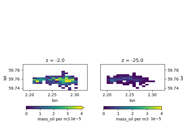
Plot the oil concentration (mass/volume, kg/m3) at depths 1-3m and 20-30m

plt.subplot(1,2,1)
cbar_kwargs={'orientation': 'horizontal', 'shrink': .9}
ds_c.mass_oil_volume_concentration.sel(z=-2).plot(vmin=0, vmax=4e-5, cbar_kwargs=cbar_kwargs)
plt.gca().set_aspect('equal', 'box')
plt.subplot(1,2,2)
ds_c.mass_oil_volume_concentration.sel(z=-25).plot(vmin=0, vmax=4e-5, cbar_kwargs=cbar_kwargs)
plt.gca().set_aspect('equal', 'box')
plt.gca().yaxis.set_label_position('right')
plt.gca().yaxis.tick_right()
plt.show()

2025-06-24 13:41:22 fv-az1280-93 matplotlib.colorbar[2414] DEBUG locator: <matplotlib.ticker.AutoLocator object at 0x7f7df3e70050>
2025-06-24 13:41:22 fv-az1280-93 matplotlib.colorbar[2414] DEBUG locator: <matplotlib.ticker.AutoLocator object at 0x7f7e02270950>

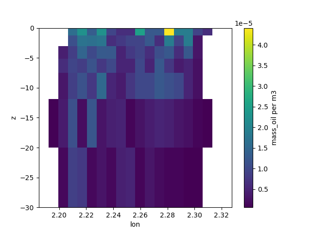
Plot a vertical profile (east to west) of the oil concentration

oil_mass_profile = ds_c.mass_oil_volume_concentration.median(dim='lat')
print(oil_mass_profile)
oil_mass_profile.plot(y='z', ylim=(None, 0))
plt.show()

<xarray.DataArray 'mass_oil_volume_concentration' (z: 7, lon: 20)> Size: 1kB
array([[           nan,            nan,            nan, 1.61433386e-05,
        2.24634651e-05, 1.32093159e-05, 2.25028758e-05, 9.56018478e-06,
        6.35711000e-06, 6.34556865e-06, 2.53085294e-05, 1.26295304e-05,
        1.26004538e-05, 4.40833430e-05, 1.88672882e-05, 1.88587364e-05,
        9.42095005e-06, 6.27488009e-06,            nan,            nan],
       [           nan,            nan,            nan, 1.12456422e-05,
        1.71172009e-05, 1.65248923e-05, 1.75570063e-05, 6.29535016e-06,
        7.85396576e-06, 9.40105090e-06, 9.38617677e-06, 1.25004533e-05,
        6.24206239e-06, 1.86967399e-05, 9.34287553e-06, 1.86680550e-05,
        3.10994094e-06,            nan,            nan,            nan],
       [           nan,            nan, 4.29393232e-06, 8.53495544e-06,
        1.45840129e-05, 1.02299643e-05, 1.27129206e-05, 1.26143276e-05,
        4.70962014e-06, 7.83817993e-06, 9.39338918e-06, 6.24710456e-06,
        1.09249917e-05, 1.24649545e-05, 6.22288049e-06, 1.24350732e-05,
        3.10737391e-06,            nan,            nan,            nan],
       [           nan,            nan, 6.21974591e-06, 9.47857881e-06,
        8.39130128e-06, 1.16747140e-05, 7.59358755e-06, 1.00796776e-05,
        5.02634607e-06, 5.01431379e-06, 1.00148937e-05, 5.00005552e-06,
        1.24830685e-05, 7.48223473e-06, 3.73840643e-06, 4.97345454e-06,
        2.48177678e-06,            nan,            nan,            nan],
       [           nan,            nan, 3.20470371e-06, 8.70677320e-06,
        1.15934087e-05, 7.74087861e-06, 1.52257931e-05, 5.13495516e-06,
        3.77248510e-06, 7.52227259e-06, 1.00186254e-05, 9.99874967e-06,
        1.24755235e-05, 1.12269865e-05, 9.96037226e-06, 4.96882284e-06,
        2.48519713e-06,            nan,            nan,            nan],
       [           nan, 8.59828075e-07, 3.72573009e-06, 1.12993297e-05,
        2.11094263e-06, 1.22746283e-05, 2.88689149e-06, 4.40413639e-06,
        4.70655434e-06, 1.25106344e-06, 2.81655742e-06, 4.06152536e-06,
        4.99421059e-06, 4.36397023e-06, 3.11456519e-06, 2.48811882e-06,
        1.24288636e-06, 6.21510547e-07,            nan,            nan],
       [           nan,            nan, 1.57117813e-06, 8.77325525e-06,
        7.80881647e-06, 1.60163967e-06, 2.84195854e-06, 1.57356884e-06,
        4.39173078e-06, 5.01259271e-06, 1.25086978e-06, 3.12287815e-06,
        1.87239539e-06, 1.24573531e-06, 1.24574803e-06, 6.22321893e-07,
        6.21260243e-07,            nan,            nan,            nan]])
Coordinates:
  * lon      (lon) float64 160B 2.189 2.196 2.203 2.21 ... 2.31 2.317 2.324
  * z        (z) float64 56B -0.505 -2.0 -4.0 -6.25 -8.75 -15.0 -25.0
Attributes:
    long_name:  mass_oil per m3
2025-06-24 13:41:22 fv-az1280-93 matplotlib.colorbar[2414] DEBUG locator: <matplotlib.ticker.AutoLocator object at 0x7f7e018f60f0>

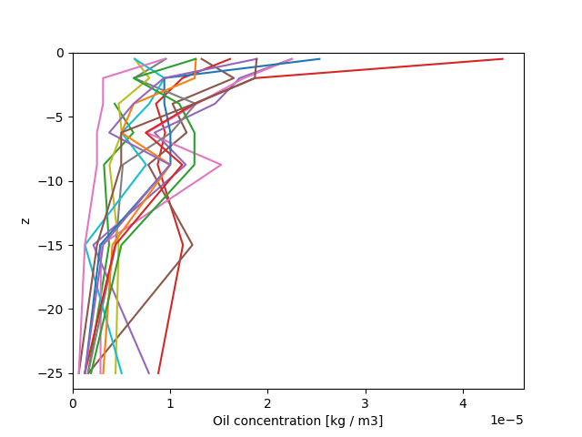
Plot the vertical profiles as lines

oil_mass_profile.plot.line(
    y='z', add_legend=False, xlim=(0, None), ylim=(None, 0))
plt.xlabel('Oil concentration [kg / m3]')
plt.show()